Determining the rate of erosion and lichen spread on Samaipata rock by comparing 3D laser scan results from two different surveying epochs

Anna Kubicka, Jacek Kościuk

doi:10.37190/arc200211

Abstract

The paper describes the possibility of using 3D laser scans from two different surveying epochs for structural health monitoring. It uses the results of two particular projects – the 2006 3D laser scanning of Samiapata rock by the University of Arkansas and the 2016 3D laser scanning by the Laboratory of 3D Laser Scanning at Wrocław University of Science and Technology – and discusses the methods, results, and limitations of comparing them.

2020

2(62)

DOI: 10.37190/arc200211

Introduction

It is becoming increasingly important to preserve and

maintain the current condition of cultural heritage sites

that have become damaged over the years due to human

and natural activity [1]. Proper preservation requires reli-

able tools that oer accurate diagnostics of current con-

ditions of the site. The latest advances in surveying tech-

nology, particularly that of 3D terrestrial laser scanning

(TLS), give the opportunity to study damage and material

decay using analysis of 3D point clouds generated by dif-

ferent instruments and techniques [2], [3]. Among them,

TLS data are widely and successfully used for structural

health monitoring in both civil engineering [4] and cultur-

al heritage [5]. This paper focuses on detecting changes to

a monument inicted by climatic erosion, human activity,

the spread of lichen, and the progress of archaeological

excavations. This monument is El Fuerte de Samaipata

– a huge sculptured rock densely covered with petro-

glyphs, niches, terraces, and platforms. The erosion oc-

curring on Samaipata rock has been addressed by earlier

studies [6]–[8] but no attempts to determinate its rate and

extent have yet been made.

Anna Kubicka*, Jacek Kościuk**

Determining the rate of erosion and lichen spread on Samaipata rock

by comparing 3D laser scan results from two different surveying epochs

Określanie stopnia erozji i tempa rozprzestrzeniania się porostów

na skale Samaipata przez porównanie wyników

skanowania laserowego 3D z dwóch różnych epok pomiarowych

In the case of Samaipata rock, the main obstacle and

dierence between similar studies of deformation meas-

urement [9], [10], [2] based on repeated TLS is the con-

siderable disparity in the parameters of the two dierent

instruments used for the scanning – the ILRIS-3D laser

scanner produced by Optech in 2006 and the ScanSta-

tion P40 introduced by Leica Geosystems in 2016. Both

scanners belong to two entirely dierent epochs of TLS

technology development; therefore, their technical char-

acteristics dier considerably.

This paper describes the three issues of 3D scanning

the Samaipata rock – the inner registration of the data

acquired in two dierent survey campaigns, the global

co-registration of the resulting two 3D point clouds, and

the methods of detecting dierences between them. Two

methods of cloud-to-cloud comparison were used to ad-

dress the last issue (“nearest neighbour distance” and “lo-

cal modeling”) in CloudCompare – an open source project

[11]. In the conclusion of this paper, we will present the

potential and limitations of analysing damage on the rock

surface using measurements collected by TLS from two

dierent sources.

Acquisition of the TLS data in 2006 and 2016

on El Fuerte de Samaipata

Due to the scale of the entire site – the Samaipata rock

itself measures 80 × 240 m and the entire site ca. 400 ×

500 m, 3D TLS was the rst choice of surveying method.

The team from the University of Arkansas collected the

* ORCID: 0000-0001-5442-3947. Faculty of Architecture, Wroc-

ław University of Science and Technology, e-mail: anna.kubicka@pwr.

edu.pl

** ORCID: 0000-0003-0623-8071. Faculty of Architecture, Wroc-

ław University of Science and Technology.

126 Anna Kubicka, Jacek Kościuk

rst TLS data of the area of sculptured rock in three days

(25–27.07.2006) [12]. The instrument used for this pur-

pose, an ILRIS-3D scanner, had a scanning range from

3 to 1200 m, a data acquisition rate of 2000 pts/sec, an

angular accuracy of 16″, and a nominal range accuracy of

7 mm @ 100 m. More details can be found at the manufac-

turer’s website [13]. The area to be scanned was covered

with 78 scan stations with an average range accuracy of

20.8 mm @ 20 m. Particular scans did not cover the full

horizontal extent but were limited to 40°/40° angular sec-

tions with typical overlap between the scans of not more

than 20–30%. This resulted in rather modest density of the

nal 3D point cloud.

Ten years after the rst survey, the team from the Labo-

ratory of 3D Scanning and Modeling covered the area of

Samaipata rock with a second TLS survey. In this case,

a Leica ScanStation P40 scanner was used. The huge pro-

gress in 3D laser scanning technology over the ten years

between the rst and the last scan resulted in considerable

improvement of the technical parameters of scanners. Al-

though the scanning range of the Leica P40 scanner was

much shorter (0.4 m to 270 m), for Samaipata rock this

had no particular impact. More critical were other param-

eters – a data acquisition rate reaching 1 mln pts/sec, an-

gular accuracy of 8″ horizontal and vertical, and nominal

range accuracy of only 1.2 mm @ 270 m. More details,

particularly on data noise, can be found at the manufac-

turer’s website [14].

Over the 14 days of eldwork, data from 278 scan sta-

tions was collected. Nearly all of the stations covered 360°

of horizontal extent, so when all of them were registered

into a common coordinate system, the density of the nal

3D point cloud was not worse than 5 × 5 mm. Over 14.5

thousand constraints were used for this registration. The

mean absolute error for constraints was 3 mm. The most

signicant errors were noticed on printed black and white

(B & W) targets attached to the platforms surrounding the

rock, which were caused by heavy vibrations from peo-

ple walking. Very strong winds also partially aected the

small tripods used for the Leica HDS targets. Weighting

was used for registration errors not exceeding 10 mm, and

in the case of more signicant errors, this constraint was

eliminated from calculations.

The referencing of all printed B & W targets to the com-

mon survey network was done with a Leica TCRP1203

Total Station. Its angular accuracy is of 3″, and the dis-

tance error is in the range of ±2 mm + 2 ppm. These

parameters, together with angular and distance observa-

tions between all pairs of mutually visible positions of

the instrument, allowed the survey network points to be

aligned with an average x, y point position square error

equal to 6.8 mm and average height square error equal to

2.9 mm.

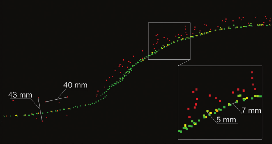
Due to the dierences between the technical speci-

cations of both scanners, the scanning parameters, and

number of scan stations, point clouds from ILRIS 3D and

Leica P40 vary in terms of point density and noise range

(Fig. 1).

Global co-registration of the point clouds

The registration of a 3D point cloud from two dierent

surveying epochs and from two dierent laser scanners

was a critical step for the whole procedure. The most pop-

ular approach, available in both CloudCompare and Leica

Cyclone software is the “Iterative Closest Point” (ICP)

Fig. 1. Section of the point cloud of a petroglyph in sector W05. Visual comparison of point cloud (6 mm width) density and noise range

between two 3D point clouds: red – ILRIS 3D (scan 2006); green – Leica P40 (scan 2016)

(elaborated by A. Kubicka)

 Determiningtherateoferosionandlichenspread / Określaniestopniaerozjiitemparozprzestrzenianiasięporostów 127

method [15]–[17]. It searches for pairs of nearest points

in two data sets and estimates the rigid body transforma-

tion that aligns them. This transformation is applied to all

points of the transformed data set, and the procedure is

repeated until required convergence is achieved [18, p. 5].

Another type of approach used in similar studies for the

global 3D cloud as well as the co-registration of surfaces

is the method of “Least Squares 3D Surface Matching”

(LS3D) [19]. On two overlapping 3D point clouds, this

method estimates the transformation parameters of one

3D cloud (or surface) with respect to a 3D template by

minimising the sum of squares of the Euclidean distanc-

es between the 3D points (or surfaces). Both methods are

widely used for the purpose of global co-registration in

studies of deformation analyses based on TLS data [9],

[10], [20], [21].

The approach proposed in this paper is also based on

the ICP method available in Leica Cyclone software for

cloud-to-cloud registration. Due to the lack of man-made

targets in the 3D point cloud from the 2006 survey, the

registration of data from separate scan stations was done

by selecting pairs of corresponding points on both 3D

clouds. At least four pairs of such points needed to be cho-

sen. Since the density of 3D clouds from the 2006 survey

was not very high, it was often dicult to nd adequately

matching pairs of points, therefore six–eight pairs were

usually chosen. In the next step, primary transformation

parameters resulting from this rough estimation were fur-

ther optimised by minimising root mean square (RMS)

error. At least 200 iterations were used.

In some cases, due to insucient overlap between scans

from 2006, it was necessary to add scans from the 2016

survey in order to merge all the data into one coherent

whole. Since the scans from 2016 were already oriented

according to our survey network, choosing one of them as

the home scanworld resulted in the same orientation of the

entire merged 3D point cloud.

Over 300 constraints were used for this registration.

The mean absolute error for constraints was below 5 mm.

Weighting was used for registration errors not exceeding

10 mm, and in the case of more signicant errors, this

constraint was eliminated from calculations.

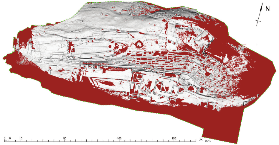
The nal results of co-registering the scans from 2006

and 2016 (Fig. 2) show dierences between the extent of

these two surveying epochs.

Methods of comparing scan results

In general, results from the two dierent surveying ep-

ochs can be compared in three ways – using only raw data

(3D point clouds), using deliverables from processing 3D

point clouds (mesh surfaces), or comparing the 3D point

clouds to meshes. All of them can be computed with the

open source software CloudCompare.

The rst method is usually called the nearest neighbour

distance. This algorithm searches for the Euclidean dis-

tance between two nearest points in both the clouds – the

reference point cloud and the point cloud being compared

[22]. For this method, the denser cloud should be used as

the reference point cloud. Only areas exactly covered by

both the scans can be directly compared. Otherwise, dis-

torted results can appear.

The second method, known as global modeling, com-

pares two surface models (meshes) derived from 3D point

clouds. For complicated and detailed surfaces, this in-

volves long computation times. Additionally, local occlu -

sions in compared data resulting in irregular triangular

meshing can again lead to erroneous results.

Fig. 2. Comparison of extents of 2006 and 2016 scans.

In grey: areas where both scans overlap, in brown: areas covered by only one scan (either 2006 or 2016)

(elaborated by A. Kubicka)

128 Anna Kubicka, Jacek Kościuk

The last method implemented in CloudCompare is

called local modeling. In this method, the dense 3D cloud

is compared to the mesh derived from the sparse point

cloud. As a result, the distance is calculated between 3D

points on the dense cloud and the nearest point lying on

the surface model as a mesh [23]. In addition to reduced

computation time, this method also results in better ap-

proximation of dierences between compared data.

Analysis of changes in the rock surface

based on data

from two different scanning epochs

Analysis involved three key steps:

– Selecting the specic areas to be analysed. These

were typically subsets of the damaged area;

– Orienting the selected area alongside the main axis,

so, for example, the vertical face corresponded to the

x–z plane;

– Estimating the deformation parameters for each se-

lected subset.

The smaller the size of the analysed area, the better

the resolution of the estimated deformations. Deforma-

tions can be analysed alongside specic axes (x, y, or z) or

globally. In the last case, the result shows only as absolute

values of dierences in Euclidean distance, without indi-

cating the dominant direction.

For analysis along one of the selected axes, it is impor-

tant to consider which of the data sets was the reference

data set and which was the compared data set. Therefore,

if, for example, the survey from 2016 was mapped as the

reference data set, negative values of deformation anal-

ysis would correspond to the declined zones of the rock

surface, and analogically, positive values would represent

material accumulated on the rock surface – mostly, prod-

ucts of rock erosion or vegetation. Reversing the mapping

would result in the opposite interpretation.

Due to the high level of noise, especially on scans from

2006, and due to the signicant dierence in the density

of scans from both surveying epochs, a distance of 0.02 m

was chosen as the threshold value for detecting defor-

mations. All results below this threshold were treated as

a side eect of the technical shortcomings of the scans. In

order to eliminate accidental data resulting from inaccu-

rate data ltration (dust particles in the air, people moving

through the area, big plants, etc.), the upper threshold for

detecting deformations was set to 0.2 m.

As the rst example of the feasibility of data sets col-

lected in the year 2006 and 2016 for analysing the pro-

gress of erosion on Samaipata rock, the front wall of a ter-

race in sector S27 will be used

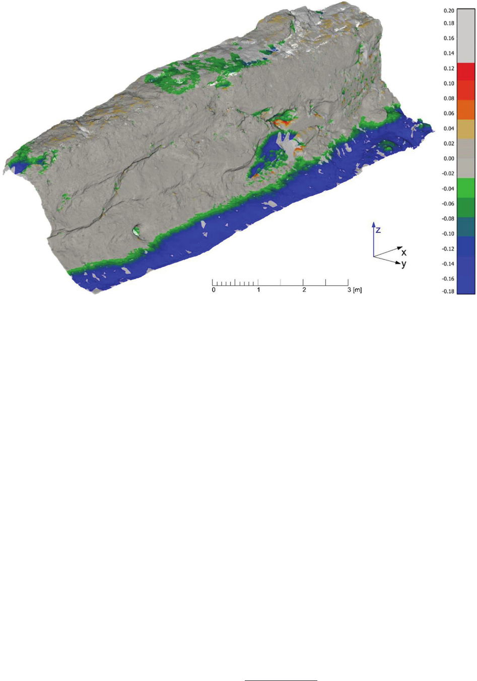
Computation of distances between two data sets an-

alysed alongside the z-axis (Fig. 3) showed particularly

signicant changes (in the range of 0.2 m) at the foot of

the vertical wall of the terrace. An analysis of excavation

logs indicates that in the years 2006–2016, archaeological

works were carried out here. However, the changes within

Cf. J. Kościuk, G. Oreci, M. Ziółkowski, A. Kubicka, R. Muñóz

Risolazo, Description and analysis of El Fuerte de Samaipata in the

lightofnewresearch,and aproposalofthe relativechronologyofits

main elements, in the same issue of “Architectus”.

Fig. 3. Part of the front wall of the terrace in sector S27. Results of deformation analysis along the z-axis

(elaborated by A. Kubicka)

 Determiningtherateoferosionandlichenspread / Określaniestopniaerozjiitemparozprzestrzenianiasięporostów 129

the terrace front wall cannot be explained by the progress

of archaeological prospection. A big cavity, an evident

place of local erosion, expanded by more than 0.2 m. Mi-

nor changes (0.02–0.06 m) observed in the upper surface

of the terrace can be attributed to rock erosion as well as

the reduction in vegetation due to the constant eorts of

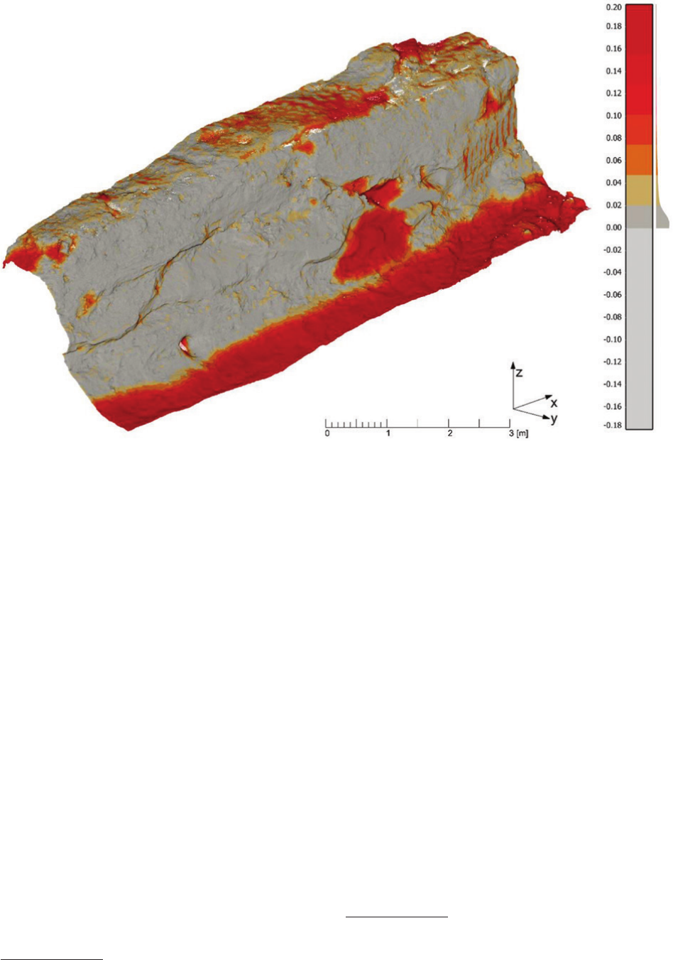
the local restoration team. These observations can be fur-

ther conrmed by global deformation analysis expressed

in absolute values (Fig. 4). In this, the erosion cavities in

the front wall are even more visible. Additionally, on the

right part of the analysed wall, traces of water erosion

(parallel vertical stripes) can be detected.

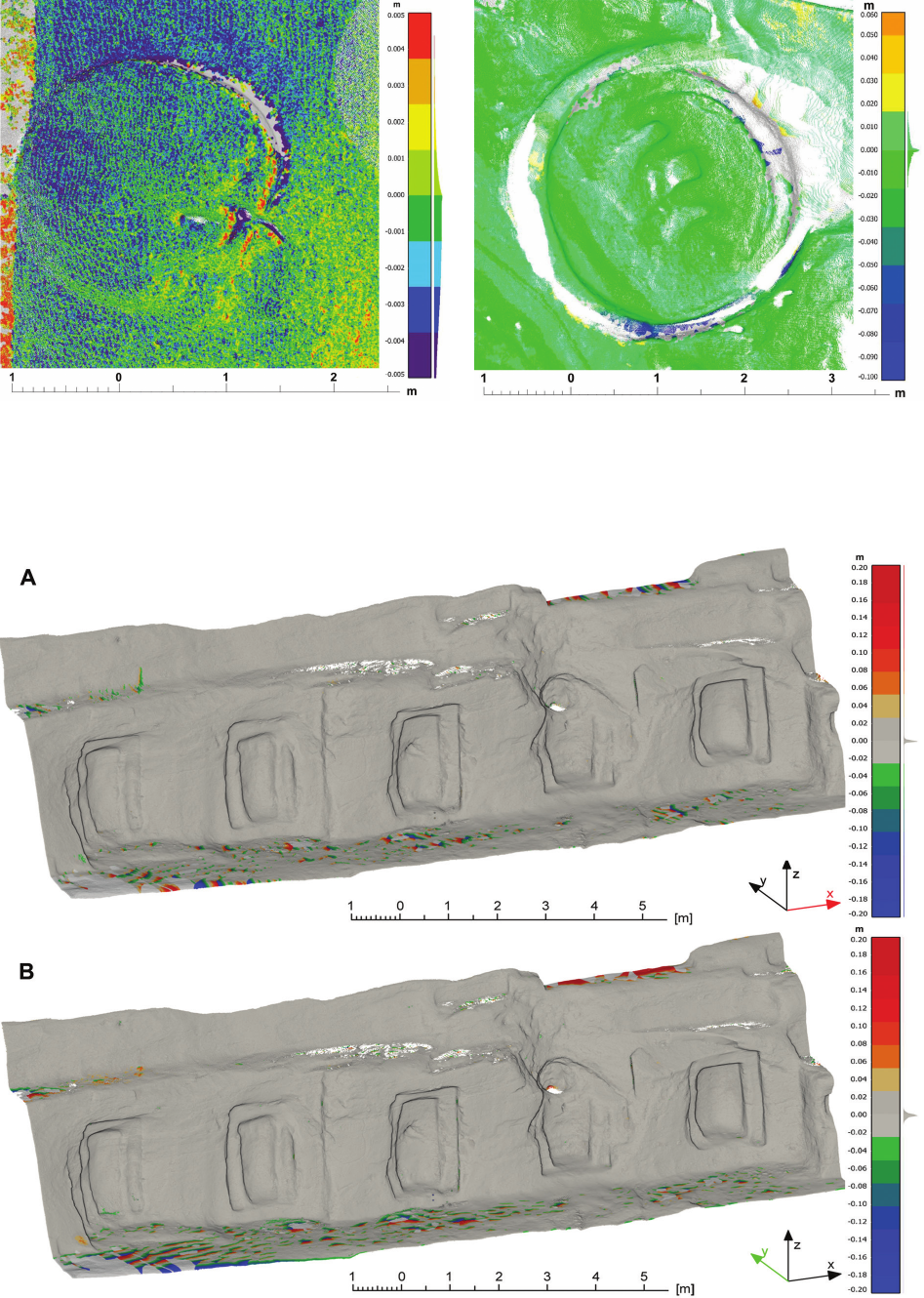
The highly eroded petroglyph

localised in sector W06

can be used as another example of detected rock erosion.

In this case, due to much smaller dierences, the upper

and the lower thresholds were set to ±0.005 m. For this

petroglyph, results of local modeling along the z-axis

(Fig. 5) show that mostly the western and northern are-

as of the petroglyph were inuenced by erosion, which

ranged from –0.003 m to –0.005 m. The positive values

alongside the south-eastern edge of the petroglyph are the

eects of growing vegetation.

Analysis of the petroglyph from sector W05 with the

clearly recognisable silhouette of a feline is a dierent

Cf. J. Kościuk, G. Oreci, M. Ziółkowski, A. Kubicka, R. Muñóz

Risolazo, Description and analysis of El Fuerte de Samaipata in the

lightofnewresearch,andaproposalof therelativechronologyofits

main elements, in the same issue of “Architectus”.

case

. There, the 3D point cloud acquired in 2006 from

the ILRIS 3D scanner has signicant noise in the range

of ±0.002 m (Fig. 6). Therefore, it was necessary to ex-

clude this range from further interpretations. Expanding

the upper and lower thresholds of deformation analysis

respectively to –0.010 and +0.06 did not bring particu-

larly useful results. A few positive anomalies (yellow and

orange spots) were caused by growing vegetation. Neg-

ative anomalies detected in a small ditch encircling the

feline gure are the results of erosion caused by water

always present in this depression. A more general obser-

vation is that the at areas where rainwater remains for

a longer period show positive anomalies (aquamarine col-

our), while more steep areas present negative anomalies

(green colour).

The possible interpretation is that positive anomalies

are associated with mosses and lichens that grow better on

more wet surfaces, while negative anomalies (on sloping

surfaces) are the result of frequent and more rapid changes

of moisture in the rock that cause the swelling and shrink-

age of smectites present

. However, due to the technical

Cf. J. Kościuk, G. Oreci, M. Ziółkowski, A. Kubicka, R. Muñóz

Risolazo, Description and analysis of El Fuerte de Samaipata in the

lightofnewresearch,andaproposalof therelativechronologyofits

main elements, in the same issue of “Architectus”.

Cf. W. Bartz, J. Kościuk, M. Gąsior, T. Dziedzic, Petrographic,

mineralogical, and climatic analyses, and risk maps for conservation

strategies, in the same issue of “Architectus”.

Fig. 4. Part of the front wall of the terrace in sector S27. Results of global deformation analysis (absolute values)

(elaborated by A. Kubicka)

130 Anna Kubicka, Jacek Kościuk

Fig. 5. Petroglyph from sector W06.

Local modeling analysis along the z-axis

(elaborated by A. Kubicka)

Fig. 6. Petroglyph from sector W05.

Local modeling analysis along the z-axis

(elaborated by A. Kubicka)

Fig. 7. The southern face of the wall with double recessed niches in sector S09:

A – local modeling analysis along the x-axis;

B – local modeling analysis along the y-axis

(elaborated by A. Kubicka)

 Determiningtherateoferosionandlichenspread / Określaniestopniaerozjiitemparozprzestrzenianiasięporostów 131

shortcomings of the acquired data, all these interpretations

should be treated with extreme caution.

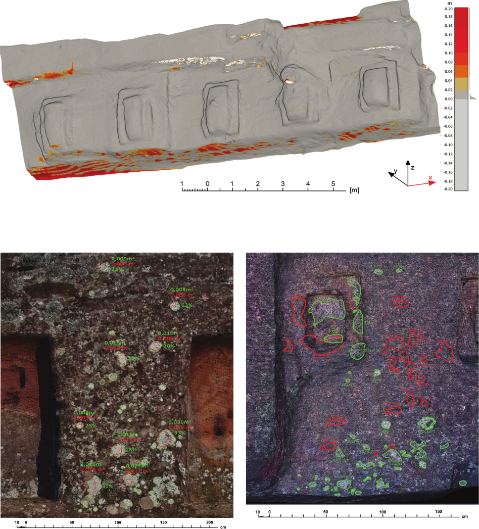
In some cases, despite eorts and searching for the best

parameters for the analysis, no signicant anomalies could

be detected. A good example is the unnished fragment of

the southern rock face with double recessed niches lying in

sector S09 (Figs. 7, 8). With the upper and lower threshold

of deformation analogous to the case of the terrace face

in sector S27 (±0.20 m), analysis according to the x-axis

(Fig. 7A), the y-axis (Fig. 7B), and the z-axis did not show

any noticeable anomalies. The only exception was the at

area in front of the niches where products of erosion (sand

and small stones) accumulated. The same results were ob-

served in the global comparison analysis (Fig. 8).

Detection and comparison of lichen spread

on the surface of the rock

Data from the 2006 and 2016 TLS surveys were also

used to detect the spread of lichen. By using dierent ren-

Fig. 8. The southern face of the wall with double recessed niches in sector S09. Global comparison analysis in absolute values

(elaborated by A. Kubicka)

Fig. 9. Wall with niches from sector S08. Orthoimage from the 3D

point cloud obtained in 2016 with information on lichen spread

in 2006 (red colour) and 2016 (green colour) (elaborated by A. Kubicka)

Fig. 10. Wall with double niches from sector S09.

Orthoimage from the 3D point cloud obtained in 2016 with information

on size of lichens in 2006 (red colour) and 2016 (green colour)

(elaborated by A. Kubicka)

132 Anna Kubicka, Jacek Kościuk

dering options and dierent parameters of 3D point cloud

visualisation, it was possible to produce natural-colour or-

thoimages sharp enough to calculate an increase, decrease,

or full extinction of lichen. Orthoimages were exported

to a CAD 2D environment and then properly scaled and

superimposed. The margins of the lichens were then on-

screen digitised and areas of each lichen were calculated.

Two specic fragments of Samaipata rock were chosen as

examples to present the results of this method.

The rst example illustrates a case in which lichens

identied in 2016 as biologically active using infrared

photographs

were analysed (Fig. 9). Compared to 2006

data, individual lichens had increased their surfaces by

20–63%. The second example illustrates a case where

over the 10 years, some lichens disappeared and new ones

started to grow (Fig. 10). Some of them, already invisible

in 2006, were able to expand to 0.65 m

in 2016.

Again, as in the case of deformation analyses, the qual-

ity of scan data played an essential role in the applicability

and accuracy of the study. Notably, the density of 3D point

data had a direct inuence on the quality of resulting or-

thoimages and therefore on the precision of the margins of

lichens on-screen digitising.

Cf. B. Ćmielewski, I. Wilczyńska, C. Patrzałek, J. Kościuk, Digi-

tal close-range photogrammetry of El Fuerte de Samaipata, in the same

issue of “Architectus”.

Conclusions: results and limitations

The general conclusion is that despite some technical

limitations resulting from the specications of scanners

from two entirely dierent stages of TLS technology

development, the method of monitoring rock erosion

and lichen spread by comparing two data sets from two

dierent surveying epochs has great potential. The other

factor that should also be taken into account is the fact

that the Arkansas team had only three days to com-

plete its eldwork [12]. The TLS survey in 2016 lasted

for 14 days, so the number of overlapping scan stations

and resulting density of data was much higher. Never-

theless, despite these limitations, it was possible to de-

tect ano malies in the range of 0.02 m and in some cases

even smaller.

Judging from the obtained results, it might be advis-

able that within the next 10 years, a TLS survey should

be repeated with specication (accuracy, density, noise)

not worse than that of 2016 – if not a scan of the whole

rock, then at least a scan of its most important fragments.

Repeated comparison of data from the other two periods

will better determine the speed of erosion and indicate the

places most exposed to it.

The use of TLS data for monitoring the state of heritage

monuments is becoming increasingly common [24], [25]

and is particularly worth recommending in the case of El

Fuerte de Samaipata.

References /Bibliografia

[1] Moropoulou A., Delegou E.T., Labropoulos K. et al., Non-destruc-

tivetechniquesasatoolfortheprotectionofbuiltculturalheritage,

“Construction and Building Materials” 2013, No. 48, 1222–1239,

doi: 10.1016/j.conbuildmat.2013.03.044.

[2] Lachat E., Landes T., Grussenmeyer P., Comparison of point cloud

registration algorithms for better result assessment – towards an

open-source solution, “The International Archives of the Photogram-

metry, Remote Sensing and Spatial Information Sciences” 2018,

Vol. XLII-2, 551–558, doi: 10.5194/isprs-archives-XLII-2-551-2018.

[3] Rabbani T., Dijkman S., van den Heuvel F. et al., An integrated ap-

proach for modelling and global registration of point clouds, “The

International Archives of the Photogrammetry, Remote Sensing and

Spatial Information Sciences” 2007, Vol. 61, Iss. 6, 355–370, doi:

10.1016/j.isprsjprs.2006.09.006.

[4] Dąbek P.B., Patrzałek C., Ćmielewski B. et al., The use of terrestrial la-

ser scanning in monitoring and analyses of erosion phenomena in nat-

ural and anthropogenically transformed areas, “Cogent Geoscience”

2018, Vol. 4, No. 1, 1–18, doi: 10.1080/23312041.2018.1437684.

[5] Selbesoglu M.O., Bakirman T., Gokbayrak O., Deformation Meas-

urement Using Terrestrial Laser Scanner for Cultural Heritage,

“The International Archives of the Photogrammetry, Remote Sens-

ing and Spatial Information Sciences” 2016, Vol. XLII-2/W1, 89–93,

doi: 10.5194/isprs-archives-XLII-2-W1-89-2016.

[6] Avilés S., ConservazionedeltempiodellaroccascolpitadiSamai-

pata–SantaCruz,Bolivia(Sudamerica), Tesi di Master, Università

di Bologna – Sede di Ravenna, Facoltà di Conservazione dei Beni

Culturali, Dipartimento di Storie e Metodi per la Conservazione dei

Beni Culturali 2002, www.stonewatch.de/media/download/sc%20

04.pdf [accessed: 1.11.2019].

[7] Avilés S., IntroduzioneallaconservazionedellaRocciaScolpitadi

Samaipata, Bolivia, 2011, http://www.rupestreweb.info/samaipata.

html [accessed: 1.11.2019].

[8] Avilés S., LaconservacióndelaRocaSagradadeSamaipata, [in:]

A. Meyers, I. Combès (comp.), El Fuerte de Samaipata. Estudios

arqueológicos, Universidad Autónoma Gabriel René Moreno, San-

ta Cruz de la Sierra 2015, 161–170.

[9] Monserrat O., Crosetto M., Deformation measurement using ter-

restriallaserscanningdataandleastsquares3Dsurfacematching,

“The International Archives of the Photogrammetry, Remote Sens-

ing and Spatial Information Sciences” 2008, Vol. 63, Iss. 1, 142–154,

doi: 10.1016/j.isprsjprs.2007.07.008.

[10] Gordon S., Lichti D., Stewart M., Applicationofahigh-resolution,

ground-based laser scanner for deformation measurements, “New

Techniques in Monitoring Surveys I, Proceedings of 10

FIG In-

ternational Symposium on Deformation Measurements” 2001,

Orange, California, 23–32, http://webarchiv.ethz.ch/geometh-data/

student/eg1/2006/14/HPLAserscanning.pdf [accessed: 20.09.2019].

[11]

CloudCompareopen-sourcesoftware, http://www.cloudcompare.org/

[accessed: 20.09.2019].

[12] Barnes A., Goodmaster C., Vranich A. et al., The El Fuerte de

Samaipata 3D Scanning Project 2005, http://www.cast.uark.edu/

samaipata/index.html [accessed: 20.09.2019].

[13] ILRIS 3D Datasheet, https://www.laserscanningeurope.com/sites/

default/les/Optech/ILRIS-Datenblatt.pdf [accessed: 20.09.2019].

[14]

Leica ScanStation P40/P30, https://leica-geosystems.com/pl-pl/

products/

laser-scanners/scanners/leica-scanstation-p40--p30 [ac-

cessed: 20.09.2019].

[15] Besl P.J., McKay M.D., A method for registration a 3D shape,

“IEEE Transactions of Pattern Analysis and Machine Intelligence”

1992, Vol. 14, Iss. 2, 239–256, doi: 10.1109/34.121791.

[16] Chen Y., Medioni G.G., ObjectModelingbyRegistrationofMul-

tipleRangeImages, “Proceedings. 1991 IEEE International Con-

ference on Robotics and Automation” 1992, Vol. 10, No. 3, 2724–

2729, doi: 10.1109/ROBOT.1991.132043.

 Determiningtherateoferosionandlichenspread / Określaniestopniaerozjiitemparozprzestrzenianiasięporostów 133

[17] Zhang Z., Iterative point matching for registration of free-form

curves and surfaces, “International Journal of Computer Vision”

1994, Vol. 13, No. 2, 119–152, doi: 10.1007/BF01427149.

[18] Akca D., LeastSquares3DSurfaceMatching, Institut für Geodä-

sie und Photogrammetrie Eidgenössische Technische Hochschule

Zürich, Zurich 2017.

[19] Gruen A., Akca D., Least Squares3D Surfaceandcurve Match-

ing, “The International Archives of the Photogrammetry, Remote

Sensing and Spatial Information Sciences” 2005, Vol. 59, Iss. 3,

151–174, doi: 10.1016/j.isprsjprs.2005.02.006.

[20] Barrile V., Meduri G.M., Bilotta G., LeastSquares3DAlgorithm

fortheStudyofDeformationswithTerrestrialLaserScanner, [in:]

V. Mladenov (ed.), Recent Advances in Electronics, Signal Pro-

cessing and Communication Systems. Proceedings of the 2013

International Conference on Electronics, Signal Processing and

Communication Systems, Venice, 2013, 162–165, https://www.

researchgate.net/publication/280731000_Least_Squares_3D_

Algorithm_for_the_Study_of_Deformations_with_Terrestrial_

Laser_Scanner [accessed: 1.11.2019].

[21] Monserrat O., Crosetto M., Pucci B., TLS deformation measure-

ment using ls3d surface and curve matching, “The International

Archives of the Photogrammetry, Remote Sensing and Spatial

Informa tion Sciences” 2008, Vol. 37, 591–596, doi: 10.1016/j.is-

prsjprs.2007.07.008.

[22] Girardeau-Montaut D., Roux M., Marc R. et al., Change detection

on point cloud data acquiredwith a ground laser scanner, [in:]

G. Vosselman, C. Brenner (eds.), ProceedingsoftheISPRSWork-

shopLaserscanning2005, ISPRSArchives, International Institute

for Geo-Information Science and Earth Observation, Enschede,

2005, Vol. 36, 30–35, https://www.isprs.org/proceedings/XXXVI/

3-W19/papers/030.pdf [accessed: 1.11.2019].

[23] https://www.cloudcompare.org/doc/wiki/index.php? title=Distanc-

es_Computation [accessed: 1.11.2019].

[24] Guarnieri A., Milan N., Vettore A., Monitoring of Complex Structure

forStructuralControlUsingTerrestrialLaserScanning(TLS)and

Photogrammetry, “International Journal of Architectural Heritage”

2013, Vol. 7, Iss. 1, 54–67, doi: 10.1080/15583058.2011.606595.

[25] Park H.S., Lee H.M., Adeli H. et al., ANewApproachforHealth

Monitoring of Structures: Terrestrial Laser Scanning, “Computer-

Aided Civil and Infrastructure Engineering” 2007, Vol. 22, Iss. 1,

19–30, doi: 10.1111/j.1467-8667.2006.00466.x.

Acknowledgements /Podziękowania

Thepresentedworkispartoftheresearchsponsoredbythegrantgiv-

entotheWrocławUniversityofScienceandTechnologybythePolish

National Science Centre (grant No. 2014/15/B/HS2/01108). Additio-

nally,themunicipalityofSamaipata,representedbyMayorFalvioLó-

pesEscalera, contributed to this researchby providingthe accommo-

dationduring the eldwork inJune and July 2016, aswell as in July

2017. The Ministry of Culture and Tourism of Bolivia kindly granted

all necessary permits (UDAM No. 014/2016; UDAM No. 060/2017).

The research was conducted in close cooperation with the Centrefor

Pre-Columbian Studies of the University of Warsaw in Cusco, Peru.

Specialists from many other universities and research centres also

joinedtheproject.Separate,butnolessimportant,thanksareowedto

the University of Arkansas for providing scan data from their survey

in2006.

Abstract

The paper describes the possibility of using 3D laser scans from two dierent surveying epochs for structural health monitoring. It uses the results of

two particular projects – the 2006 3D laser scanning of Samiapata rock by the University of Arkansas and the 2016 3D laser scanning by the Labora-

tory of 3D Laser Scanning at Wrocław University of Science and Technology – and discusses the methods, results, and limitations of comparing them.

Key words: El Fuerte de Samaipata, Bolivia, terrestrial laser scanning, cloud-to-cloud comparison, structural health monitoring

Streszczenie

W artykule opisano możliwość zastosowania laserowego skanowania 3D z dwóch różnych epok pomiarowych do monitorowania stanu zabytku.

Wykorzystano wyniki wykonanego przez University of Arkansas laserowego skanowania El Fuerte de Samaipata z 2006 r. oraz laserowego skanowa-

nia 3D z roku 2016 wykonanego przez Laboratorium Skanowania Laserowego 3D Politechniki Wrocławskiej. Omówiono wyniki i ograniczenia

proponowanej metody.

Słowa kluczowe: El Fuerte de Samaipata, Boliwia, naziemne skanowanie laserowe, cloud-to-cloud comparison, monitorowanie stanu zabytku

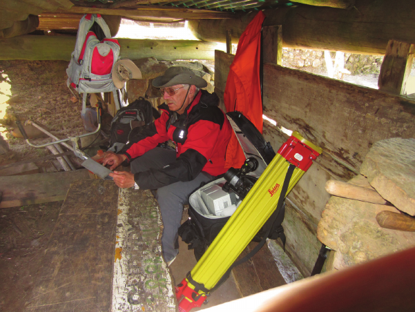
Checking data collected of the field

(photo by M. Telesińska)

Sprawdzanie zebranych danych

(fot. M. Telesińska)